DIVERGING-WAVE ECHOCARDIOGRAPHY - simulations, beamforming, compounding
In this tutorial, it is shown how to simulate an ultrasound image of the heart (a five-chamber view) from the transmit of diverging waves.
The heart will be insonified with seven diverging waves 60-degrees wide.
- Scatterers will be provided by the function GENSCAT.
- RF signals will be simulated with the function SIMUS.
- The RF signals will be I/Q demodulated with RF2IQ,
- then beamformed with DAS.
- A compound echocardiographic image will eventually be generated.
Contents
- Select a transducer with GETPARAM
- Add transmit apodization
- Set the transmit delays with TXDELAY
- Simulate an acoustic pressure field with PFIELD
- Simulate RF signals with SIMUS
- Demodulate the RF signals with RF2IQ
- Beamform the I/Q signals with DAS
- Time-gain compensate the beamformed I/Q with TGC
- Check the ultrasound images
- See also
- About the author
- Date modified
Select a transducer with GETPARAM
We want a 2.7-MHz 64-element cardiac phased array.
param = getparam('P4-2v');
The structure param contains the tranducer properties.
Add transmit apodization
param.TXapodization = cos(linspace(-1,1,64)*pi/2);
Set the transmit delays with TXDELAY
The left ventricle will be insonified with seven diverging waves 60 degrees wide and tilted at -20 to +20 degrees.
tilt = deg2rad(linspace(-20,20,7)); % tilt angles in rad
txdel = cell(7,1); % this cell will contain the transmit delays
Use TXDELAY to calculate the transmit delays for the 7 diverging waves.
for k = 1:7
    txdel{k} = txdelay(param,tilt(k),deg2rad(60));
end
These are the transmit delays to obtain a 60 degrees wide circular waves steered at -20 degrees
stem(txdel{1}*1e6)
xlabel('Element number')
ylabel('Delays (\mus)')
title('TX delays for a 60{\circ}-wide -20{\circ}-tilted wave')
axis tight square

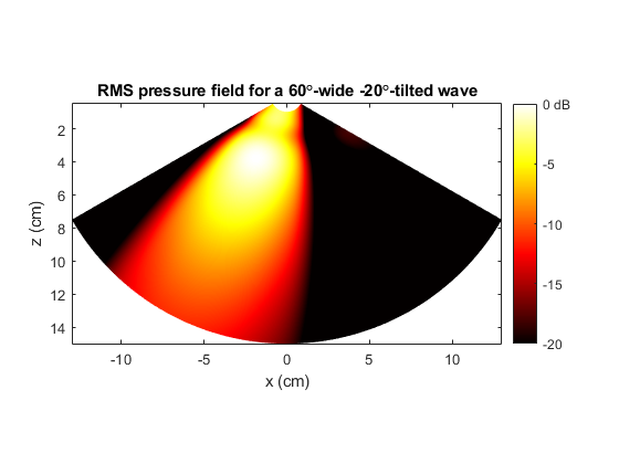
Simulate an acoustic pressure field with PFIELD
Check what the sound pressure fields look like.
Define a 100  100 polar grid using IMPOLGRID:
[xi,zi] = impolgrid([100 100],15e-2,deg2rad(120),param);
Simulate an RMS pressure field...
option.WaitBar = false;
P = pfield(xi,0*xi,zi,txdel{1},param,option);
...and display the result:
pcolor(xi*1e2,zi*1e2,20*log10(P/max(P(:))))
shading interp
xlabel('x (cm)')
ylabel('z (cm)')
title('RMS pressure field for a 60{\circ}-wide -20{\circ}-tilted wave')
axis equal ij tight
caxis([-20 0]) % dynamic range = [-20,0] dB
cb = colorbar;
cb.YTickLabel{end} = '0 dB';
colormap(hot)
Simulate RF signals with SIMUS
We will now simulate seven series of RF signals. Each series will contain 64 RF signals, as the simulated phased array contains 64 elements. We first create scatterers with GENSCAT from a clipart image of the ventricle stored in heart.jpg.
x, y, and z contain the scatterers' positions. RC contains the reflection coefficients.
I = rgb2gray(imread('heart.jpg'));
% Pseudorandom distribution of scatterers (depth is 15 cm)
[x,y,z,RC] = genscat([NaN 15e-2],1540/param.fc,I);
Take a look at the scatterers. The backscatter coefficients are gamma-compressed to increase the contrast.
scatter(x*1e2,z*1e2,2,abs(RC).^.25,'filled')
colormap([1-hot;hot])
axis equal ij tight
set(gca,'XColor','none','box','off')
title('Scatterers for a cardiac 5-chamber view')
ylabel('[cm]')

Simulate the seven series of RF signals with SIMUS. The RF signals will be sampled at 4 center frequency.
RF = cell(7,1); % this cell will contain the RF series
param.fs = 4*param.fc; % sampling frequency in Hz

option.WaitBar = false; % remove the wait bar of SIMUS
h = waitbar(0,'');
for k = 1:7
    waitbar(k/7,h,['SIMUS: RF series #' int2str(k) ' of 7'])
    RF{k} = simus(x,y,z,RC,txdel{k},param,option);
end
close(h)
This is the 32th RF signal of the 1st series:
rf = RF{1}(:,32);
t = (0:numel(rf)-1)/param.fs*1e6; % time (ms)
plot(t,rf)
set(gca,'YColor','none','box','off')
xlabel('time (\mus)')
title('RF signal of the 32^{th} element (1^{st} series, tilt = -20{\circ})')
axis tight

Demodulate the RF signals with RF2IQ
Before beamforming, the RF signals must be I/Q demodulated.
IQ = cell(7,1);  % this cell will contain the I/Q series

for k = 1:7
    IQ{k} = rf2iq(RF{k},param.fs,param.fc);
end
This is the 32th I/Q signal of the 1st series:
iq = IQ{1}(:,32);
plot(t,real(iq),t,imag(iq))
set(gca,'YColor','none','box','off')
xlabel('time (\mus)')
title('I/Q signal of the 32^{th} element (1^{st} series, tilt = -20{\circ})')
legend({'in-phase','quadrature'})
axis tight

Beamform the I/Q signals with DAS
To generate images of the left ventricle, beamform the I/Q signals onto a 256 128 polar grid.
Generate the image (polar) grid using IMPOLGRID.
[xi,zi] = impolgrid([256 128],15e-2,deg2rad(80),param);
Beamform the I/Q signals using a delay-and-sum with the function DAS.
bIQ = zeros(256,128,7);  % this array will contain the 7 I/Q images

h = waitbar(0,'');
for k = 1:7
    waitbar(k/7,h,['DAS: I/Q series #' int2str(k) ' of 7'])
    bIQ(:,:,k) = das(IQ{k},xi,zi,txdel{k},param);
end
close(h)
Time-gain compensate the beamformed I/Q with TGC
Time-gain compensation tends to equalize the amplitudes along fast-time.
bIQ = tgc(bIQ);
Check the ultrasound images
An ultrasound image is obtained by log-compressing the amplitude of the beamformed I/Q signals. Have a look at the images obtained when steering at -20 degrees.
I = bmode(bIQ(:,:,1),50); % log-compressed image
pcolor(xi*1e2,zi*1e2,I)
shading interp, colormap gray
title('DW-based echo image with a tilt angle of -20{\circ}')

axis equal ij
set(gca,'XColor','none','box','off')
c = colorbar;
c.YTick = [0 255];
c.YTickLabel = {'-50 dB','0 dB'};
ylabel('[cm]')

The individual images are of poor quality. The compound image obtained with a series of 7 diverging waves steered at different angles is of better quality:
cIQ = sum(bIQ,3); % this is the compound beamformed I/Q
I = bmode(cIQ,50); % log-compressed image
pcolor(xi*1e2,zi*1e2,I)
shading interp, colormap gray
title('Compound DW-based cardiac echo image')

axis equal ij
set(gca,'XColor','none','box','off')
c = colorbar;
c.YTick = [0 255];
c.YTickLabel = {'-50 dB','0 dB'};
ylabel('[cm]')

See also
About the author
Damien Garcia, Eng., Ph.D.
INSERM researcher
Creatis, University of Lyon, France
websites: BioméCardio, MUST
Date modified