SMOOTHN - Robust spline smoothing for 1-D to N-D data

SMOOTHN provides a fast, automatized and robust discretized spline smoothing for data of arbitrary dimension.

Z = SMOOTHN(Y) automatically smoothes the uniformly-sampled array Y. Y can be any N-D noisy array (time series, images, 3D data,...). Non finite data (NaN or Inf) are treated as missing values.

Z = SMOOTHN(Y,S) smoothes the array Y using the smoothing parameter S. S must be a real positive scalar. The larger S is, the smoother the output will be. If the smoothing parameter S is omitted (see previous option) or empty (i.e. S = []), it is automatically determined by minimizing the generalized cross-validation (GCV) score.

Z = SMOOTHN(Y,W) or Z = SMOOTHN(Y,W,S) smoothes Y using a weighting array W of positive values, which must have the same size as Y. Note that a nil weight corresponds to a missing value.

[Z,S] = SMOOTHN(...) also returns the calculated value for the smoothness parameter S so that you can fine-tune the smoothing subsequently if needed.

Contents

Smoothing vector fields or multi-component data

If you want to smooth a vector field or multicomponent data, Y must be a cell array. For example, if you need to smooth a 3-D vectorial flow (Vx,Vy,Vz), use Y = {Vx,Vy,Vz}. The output Z is also a cell array which contains the smoothed components. See examples below.

Robust smoothing

Z = SMOOTHN(...,'robust') carries out a robust smoothing that minimizes the influence of outlying data.

An iteration process is used with the 'ROBUST' option, or in the presence of weighted and/or missing values. Z = SMOOTHN(...,OPTIONS) smoothes with the termination parameters specified in the structure OPTIONS. OPTIONS is a structure of optional parameters that change the default smoothing properties. It must be the last input argument.

The structure OPTIONS can contain the following fields:

[Z,S,EXITFLAG] = SMOOTHN(...) returns a boolean value EXITFLAG that describes the exit condition of SMOOTHN; 1: SMOOTHN converged, 0: Maximum number of iterations was reached.

Different spacing increments

SMOOTHN, by default, assumes that the spacing increments are constant and equal in all the directions (i.e. dx = dy = dz = ...). This means that the smoothness parameter is also similar for each direction. If the increments differ from one direction to the other, it can be useful to adapt these smoothness parameters. You can thus use the following field in OPTIONS:

Important note: d1 is the spacing increment for the first non-singleton dimension (i.e. the vertical direction for matrices).

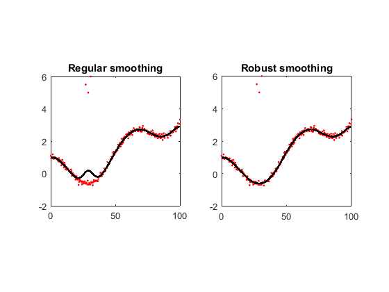
Example #1: smooth a curve

x = linspace(0,100,2^8);
y = cos(x/10)+(x/50).^2 + randn(size(x))/10;
y([70 75 80]) = [5.5 5 6];
z = smoothn(y); % Regular smoothing
zr = smoothn(y,'robust'); % Robust smoothing
subplot(121), plot(x,y,'r.',x,z,'k','LineWidth',2)
axis square, title('Regular smoothing')
subplot(122), plot(x,y,'r.',x,zr,'k','LineWidth',2)
axis square, title('Robust smoothing')

Example #2: smooth a surface

xp = 0:.02:1;
[x,y] = meshgrid(xp);
f = exp(x+y) + sin((x-2*y)*3);
fn = f + randn(size(f))*0.5;
fs = smoothn(fn);
subplot(121), surf(xp,xp,fn), zlim([0 8]), axis square
subplot(122), surf(xp,xp,fs), zlim([0 8]), axis square

Example #3: smooth 2-D data with missing values

n = 256;
y0 = peaks(n);
y = y0 + randn(size(y0))*2;
I = randperm(n^2);
y(I(1:n^2*0.5)) = NaN; % lose 1/2 of data
y(40:90,140:190) = NaN; % create a hole
z = smoothn(y); % smooth data
subplot(2,2,1:2), imagesc(y), axis equal off
title('Noisy corrupt data')
subplot(223), imagesc(z), axis equal off
title('Recovered data ...')
subplot(224), imagesc(y0), axis equal off
title('... compared with the actual data')

Example #4: smooth volumetric data

[x,y,z] = meshgrid(-2:.2:2);
xslice = [-0.8,1]; yslice = 2; zslice = [-2,0];
vn = x.*exp(-x.^2-y.^2-z.^2) + randn(size(x))*0.06;
subplot(121), slice(x,y,z,vn,xslice,yslice,zslice,'cubic')
axis square
title('Noisy data')
v = smoothn(vn);
subplot(122), slice(x,y,z,v,xslice,yslice,zslice,'cubic')
axis square
title('Smoothed data')

Example #5: smooth a cardioid

t = linspace(0,2*pi,1000);
x = 2*cos(t).*(1-cos(t)) + randn(size(t))*0.1;
y = 2*sin(t).*(1-cos(t)) + randn(size(t))*0.1;
z = smoothn({x,y});
figure
plot(x,y,'r.',z{1},z{2},'k','linewidth',2)
axis equal tight

Example #6: smooth a 3-D parametric curve

t = linspace(0,6*pi,1000);
x = sin(t) + 0.1*randn(size(t));
y = cos(t) + 0.1*randn(size(t));
z = t + 0.1*randn(size(t));
u = smoothn({x,y,z});
figure
plot3(x,y,z,'r.',u{1},u{2},u{3},'k','linewidth',2)
axis tight square

Example #7: smooth a 2-D vector field

[x,y] = meshgrid(linspace(0,1,24));
Vx = cos(2*pi*x+pi/2).*cos(2*pi*y);
Vy = sin(2*pi*x+pi/2).*sin(2*pi*y);
Vx = Vx + sqrt(0.05)*randn(24,24); % adding Gaussian noise
Vy = Vy + sqrt(0.05)*randn(24,24); % adding Gaussian noise
I = randperm(numel(Vx));
Vx(I(1:30)) = (rand(30,1)-0.5)*5; % adding outliers
Vy(I(1:30)) = (rand(30,1)-0.5)*5; % adding outliers
Vx(I(31:60)) = NaN; % missing values
Vy(I(31:60)) = NaN; % missing values
Vs = smoothn({Vx,Vy},'robust'); % automatic smoothing
subplot(121), quiver(x,y,Vx,Vy,2.5), axis square off tight
title('Noisy velocity field')
subplot(122), quiver(x,y,Vs{1},Vs{2}), axis square off tight
title('Smoothed velocity field')

Example #8: smooth a 3-D vector field

Load data and make them noisy

load wind % original 3-D flow
% Gaussian noise
un = u + randn(size(u))*8;
vn = v + randn(size(v))*8;
wn = w + randn(size(w))*8;
% Add some outliers
I = randperm(numel(u)) < numel(u)*0.025;
un(I) = (rand(1,nnz(I))-0.5)*200;
vn(I) = (rand(1,nnz(I))-0.5)*200;
wn(I) = (rand(1,nnz(I))-0.5)*200;

Visualize the noisy flow (see CONEPLOT documentation)

figure, title('Noisy 3-D vectorial flow')
xmin = min(x(:)); xmax = max(x(:));
ymin = min(y(:)); ymax = max(y(:));
zmin = min(z(:));
daspect([2,2,1])
xrange = linspace(xmin,xmax,8);
yrange = linspace(ymin,ymax,8);
zrange = 3:4:15;
[cx,cy,cz] = meshgrid(xrange,yrange,zrange);
k = 0.1;
hcones = coneplot(x,y,z,un*k,vn*k,wn*k,cx,cy,cz,0);
set(hcones,'FaceColor','red','EdgeColor','none')
hold on
wind_speed = sqrt(un.^2 + vn.^2 + wn.^2);
hsurfaces = slice(x,y,z,wind_speed,[xmin,xmax],ymax,zmin);
set(hsurfaces,'FaceColor','interp','EdgeColor','none')
hold off
axis tight; view(30,40); axis off
camproj perspective; camzoom(1.5)
camlight right; lighting phong
set(hsurfaces,'AmbientStrength',.6)
set(hcones,'DiffuseStrength',.8)

Smooth the noisy flow and display the result

Vs = smoothn({un,vn,wn},'robust');
figure, title('3-D flow smoothed by SMOOTHN')
daspect([2,2,1])
hcones = coneplot(x,y,z,Vs{1}*k,Vs{2}*k,Vs{3}*k,cx,cy,cz,0);
set(hcones,'FaceColor','red','EdgeColor','none')
hold on
wind_speed = sqrt(Vs{1}.^2 + Vs{2}.^2 + Vs{3}.^2);
hsurfaces = slice(x,y,z,wind_speed,[xmin,xmax],ymax,zmin);
set(hsurfaces,'FaceColor','interp','EdgeColor','none')
hold off
axis tight; view(30,40); axis off
camproj perspective; camzoom(1.5)
camlight right; lighting phong
set(hsurfaces,'AmbientStrength',.6)
set(hcones,'DiffuseStrength',.8)

Pick of the week in Matlab FEX

Smooth your data

References

Please refer to the two following papers:

See also

inpaintn, evar

About the author

Damien Garcia, Eng., Ph.D.
INSERM researcher
Creatis, University of Lyon, France

website: BioméCardio

Published with MATLAB® R2017a