IQ2DOPPLER I/Q data to color Doppler
IQ2DOPPLER converts I/Q data to Doppler velocities.
Contents
Syntax
VD = IQ2DOPPLER(IQ,PARAM) returns the Doppler velocities from the I/Q time series using a slow-time autocorrelator.
PARAM is a structure that must contain the following fields:
- PARAM.fc: center frequency (in Hz, required)
- PARAM.c: longitudinal velocity (in m/s, default = 1540 m/s)
- PARAM.PRF (in Hz) or PARAM.PRP (in s): pulse repetition frequency or period (required)
VD = IQ2DOPPLER(IQ,PARAM,M):
- If M is of a two-component vector [M(1) M(2)], the output Doppler velocity is estimated from the M(1) -by- M(2) neighborhood around the corresponding pixel.
- If M is a scalar, then an M -by- M neighborhood is used.
- If M is empty, then M = 1. This is the default.
VD = IQ2DOPPLER(IQ,PARAM,M,LAG) uses a lag of value LAG in the autocorrelator. By default, LAG = 1.
[VD,VarD] = IQ2DOPPLER(...) also returns an estimated Doppler variance.
Important note
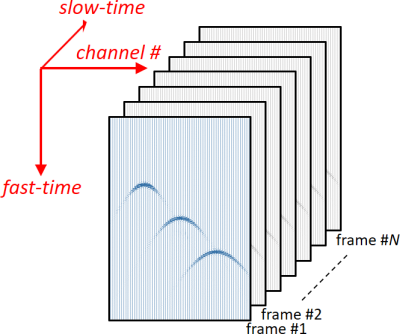
IQ must be a 3-D complex array, where the real and imaginary parts correspond to the in-phase and quadrature components, respectively. The 3rd dimension corresponds to the slow-time axis.
IQ2DOPPLER uses a full ensemble length to perform the auto-correlation, i.e. ensemble length (or packet size) = size(IQ,3).
Example #1: Color Doppler with plane wave imaging
This example shows how to obtain color Doppler velocities from RF signals acquired by plane wave imaging.
A rotating disk (diameter of 2 cm) was insonified by a series of 32 unsteered plane waves with a Verasonics scanner, and a linear transducer, at a PRF (pulse repetition frequency) of 10 kHz. The RF signals were downsampled at 4/3  (5 MHz) = 6.66 MHz. The properties of the linear array were:
- 128 elements
- center frequency = 5 MHz
- pitch = 0.298 mm
Download the experimental RF data. The 3-D array RF contains 128 columns (as the transducer contained 128 elements), and its length is 32 in the third dimension (as 32 plane waves were transmitted).
load('PWI_disk.mat')
The structure param contains some experimental properties that are required for the following steps.
disp('''param'' is a structure whose fields are:')
disp(param)
'param' is a structure whose fields are:
           fs: 6.6667e+06
        pitch: 2.9800e-04
           fc: 5000000
            c: 1480
           t0: 9.9500e-06
          PRF: 10000
        width: 2.6200e-04
    Nelements: 128
      TXdelay: [0 0 0 0 0 0 0 0 0 0 0 0 0 0 0 0 0 0 0 0 0 0 0 0 0 0 0 0 0 … ]
    bandwidth: 15
Demodulate the RF signals with RF2IQ.
IQ = rf2iq(RF,param);
Create a 2.5-cm-by-2.5-cm image grid.
dx = 1e-4; % grid x-step (in m)
dz = 1e-4; % grid z-step (in m)
[x,z] = meshgrid(-1.25e-2:dx:1.25e-2,1e-2:dz:3.5e-2);
Create a Delay-And-Sum DAS matrix with DASMTX.
param.fnumber = []; % an f-number will be determined by DASMTX
M = dasmtx(1i*size(IQ),x,z,param,'nearest');
spy(M)
axis square
title('The sparse DAS matrix')

Beamform the I/Q signals.
The 32 I/Q series can be beamformed simultaneously with the DAS matrix.
IQb = M*reshape(IQ,[],32);
IQb = reshape(IQb,[size(x) 32]);
Create and display an ultrasound image with BMODE.
B = bmode(IQb(:,:,1),30); % log-compressed image

imagesc(x(1,:)*100,z(:,1)*100,B)
c = colorbar;
c.YTick = [0 255];
c.YTickLabel = {'-30 dB','0 dB'};
colormap gray
title('B-mode image of the 1^{st} frame')
ylabel('[cm]')
shading interp
axis equal ij tight
set(gca,'XColor','none','box','off')

Calculate the Doppler velocities by using IQ2DOPPLER.
Vd = iq2doppler(IQb,param,[11 11]);
Display the color Doppler map
imagesc(x(1,:)*100,z(:,1)*100,Vd)
colormap dopplermap
colorbar
caxis([-1 1]*max(abs(Vd(:))))
title('Color Doppler map of the rotating disk')
ylabel('[cm]')
axis equal ij tight
set(gca,'XColor','none','box','off')

Display the power Doppler map.
P = sum(abs(IQb).^2,3); % power Doppler
P = 20*log10(P/max(P(:))); % log-compressed power Doppler
imagesc(x(1,:)*100,z(:,1)*100,P)
caxis([-40 0]) % dynamic range = [-40,0] dB
c = colorbar;
c.YTickLabel{end} = '0 dB';
colormap hot
title('Power Doppler map of the rotating disk')
ylabel('[cm]')
axis equal ij tight
set(gca,'XColor','none','box','off')

Create a ROI to get a masked color Doppler.
idx = P>-40;
xc = mean(x(idx)); zc = mean(z(idx)); % center of the disk
R = sqrt(nnz(idx)*dx*dz/pi); % estimated radius
roi = hypot(x-xc,z-zc)<R; % binary mask
Display a nicer color Doppler.
Vd(~roi) = 0; % discard the out-of-ROI velocities
imagesc(x(1,:)*100,z(:,1)*100,Vd)
colormap dopplermap
colorbar
caxis([-1 1]*max(abs(Vd(:))))
title('Color Doppler map of the rotating disk')
ylabel('[cm]')
axis equal ij tight
set(gca,'XColor','none','box','off')

Example #2: Vector Doppler with plane wave imaging
This example shows how to make vector Doppler imaging from RF signals acquired by plane wave imaging.
A rotating disk (diameter of 2 cm) was insonified by a series of 32 unsteered plane waves with a Verasonics scanner, and a linear transducer, at a PRF (pulse repetition frequency) of 10 kHz. The RF signals were downsampled at 4/3 (5 MHz) = 6.66 MHz. The properties of the linear array were:
- 128 elements
- center frequency = 5 MHz
- pitch = 0.298 mm
Download the experimental RF data. The 3-D array RF contains 128 columns (as the transducer contained 128 elements), and its length is 32 in the third dimension (as 32 plane waves were transmitted).
load('PWI_disk.mat');
The structure param contains some experimental properties that are required for the following steps.
disp('''param'' is a structure whose fields are:')
disp(param)
'param' is a structure whose fields are:
           fs: 6.6667e+06
        pitch: 2.9800e-04
           fc: 5000000
            c: 1480
           t0: 9.9500e-06
          PRF: 10000
        width: 2.6200e-04
    Nelements: 128
      TXdelay: [0 0 0 0 0 0 0 0 0 0 0 0 0 0 0 0 0 0 0 0 0 0 0 0 0 0 0 0 0 … ]
    bandwidth: 15
Demodulate the RF signals with RF2IQ.
IQ = rf2iq(RF,param);
Create a 2.5-cm-by-2.5-cm image grid.
dx = 1e-4; % grid x-step (in m)
dz = 1e-4; % grid z-step (in m)
[x,z] = meshgrid(-1.25e-2:dx:1.25e-2,1e-2:dz:3.5e-2);
Create a Delay-And-Sum DAS matrix with DASMTX.
Two receive angles of  are used for vector Doppler.
An adequate f-number must be chosen.
param.fnumber = [];

param.RXangle = pi/12; % receive angle (in rad)
Mp = dasmtx(1i*size(IQ),x,z,param); % DAS matrix for +15 degrees

param.RXangle = -pi/12; % receive angle (in rad)
Mm = dasmtx(1i*size(IQ),x,z,param); % DAS matrix for -15 degrees
Beamform the I/Q signals twice (at  and
and  ).
).
IQp = Mp*reshape(IQ,[],32);
IQp = reshape(IQp,[size(x) 32]);

IQm = Mm*reshape(IQ,[],32);
IQm = reshape(IQm,[size(x) 32]);
Calculate the Doppler velocities by using IQ2DOPPLER.
Vp = iq2doppler(IQp,param,[11 11]); % at +15 degrees
Vm = iq2doppler(IQm,param,[11 11]); % at -15 degrees
Display the two color Doppler maps.
subplot(121)
imagesc(Vp)
colormap dopplermap
caxis([-1 1]*max(abs(Vp(:))))
title('Color Doppler at +15^{\circ}')
axis equal ij off

subplot(122)
imagesc(Vm)
colormap dopplermap
caxis([-1 1]*max(abs(Vm(:))))
title('Color Doppler at -15^{\circ}')
axis equal ij off

Create a ROI to get masked color Doppler.
roi = hypot(x,z-.023)<.01; % binary mask

Vp(~roi) = NaN; % discard the out-of-ROI velocities
Vm(~roi) = NaN; % discard the out-of-ROI velocities
Calculate the x- and z-components of the velocity vectors.
Vx = (Vm-Vp)/sind(15);
Vz = -(Vm+Vp)/(1+cosd(15));
Display the velocity vector map.
figure
vplot(x*100,z*100,Vx,Vz)
ylabel('[cm]')
axis equal ij tight
set(gca,'XColor','none','box','off')
maxV = max(hypot(Vz,Vz),[],'all'); % maximum velocity
caxis([0 0.9*maxV])
c = colorbar;
c.YTickLabel{1} = '0 m/s';
colormap(flipud(hot))
title('Vector Doppler without smoothing')

Smooth the vector Doppler map by using SMOOTHN.
Vs = smoothn({Vx,Vz},1e4,'robust');
Vs{1}(~roi) = NaN;
Vs{2}(~roi) = NaN;
Display a smoothed velocity vector map.
figure
vplot(x*100,z*100,Vs{1},Vs{2})
ylabel('[cm]')
axis equal ij tight
set(gca,'XColor','none','box','off')
maxV = max(hypot(Vs{1},Vs{2}),[],'all'); % maximum velocity
caxis([0 0.9*maxV])
c = colorbar;
c.YTickLabel{1} = '0 m/s';
colormap(flipud(hot))
title('Vector Doppler by plane wave imaging')

See also
rf2iq, dopplermap, wfilt, dasmtx
Reference
- Madiena C, Faurie J, Poree J, Garcia D. Color and vector flow imaging in parallel ultrasound with sub-Nyquist sampling. IEEE Trans Ultrason Ferroelectr Freq Control, 2018;65:795-802. (PDF)
About the author
Damien Garcia, Eng., Ph.D.
INSERM researcher
Creatis, University of Lyon, France
websites: BioméCardio, MUST
Date modified