PFIELD3 3-D RMS acoustic pressure field of a planar array
PFIELD3 returns the three-dimensional radiation pattern of a planar 2-D array
Contents
- Syntax
- Planar 2-D array
- The structure PARAM
- Other syntaxes
- X-, Y-, and Z-axes
- Element directivity
- Present version of PFIELD3
- PFIELD vs. PFIELD3
- Note on CHIRP signals
- Advanced options
- Example #1: 3-D focused pressure field with a matrix-array transducer
- Example #2: 3-D pressure field focused on a line
- Example #3: Plane wave with a matrix array
- Example #4: Double-focus-line transmit with a matrix-array
- Example #5: 3-D diverging wave with a matrix array
- See also
- References
- About the author
- Date modified
Syntax
RP = PFIELD3(X,Y,Z,DELAYS,PARAM) returns the three-dimensional radiation pattern of a planar 2-D array whose elements are excited at different time delays (given by the vector DELAYS). The radiation pattern RP is given in terms of the root-mean-square (RMS) of acoustic pressure. The characteristics of the array and transmission must be given in the structure PARAM. The x- and y-coordinates of the elements must be in PARAM.elements (see below for details). The radiation pattern is calculated at the points specified by (X,Y,Z).
Consider using TXDELAY3 to create the vector DELAYS with standard delays (focus point, focus line, plane waves, diverging waves) with a matrix array.
Use PFIELD for uniform linear or convex arrays.
TRY IT! Enter pfield3 in the command window for an example.
Units: X, Y, Z must be in m; DELAYS must be in s.
DELAYS can be a matrix. This syntax can be used to simulate MPT (multi-plane transmit) sequences, for example. In this case, each ROW represents a delay series. For example, to create a 3-MPT sequence with a 1024-element matrix array, the DELAYS matrix must have 3 rows and
PFIELD3 is called by SIMUS3 to simulate ultrasound RF radio-frequency signals generated by a planar 2-D array.
Planar 2-D array
The present version of PFIELD3 only considers planar 2-D array whose z-coordinates of the elements are 0. All the elements are rectangular and have equal width and height.
The element width and height are both required as input parameters for PFIELD3. The element See the paragraph below entitled The structure PARAM for details.
The structure PARAM
PARAM is a structure that contains the following fields:
- TRANSDUCER PROPERTIES
- PARAM.fc: central frequency (in Hz, required)
- PARAM.elements: x- and y-coordinates of the element centers (in m, required). It MUST be a two-row matrix, with the 1st and 2nd rows containing the x and y coordinates, respectively.
- PARAM.width: element width, in the x-direction (in m, required)
- PARAM.height: element height, in the y-direction (in m, required)
- PARAM.bandwidth: pulse-echo (2-way) 6dB fractional bandwidth (in %). The default is 75%.
- PARAM.baffle: property of the baffle: 'soft' (default), 'rigid' or a scalar > 0. See Note on BAFFLE property in pfield for details.
- MEDIUM PARAMETERS
- PARAM.c: longitudinal velocity (in m/s, default = 1540 m/s)
- PARAM.attenuation: attenuation coefficient (dB/cm/MHz, default: 0). A linear frequency-dependence is assumed. A typical value for soft tissues is ~0.5 dB/cm/MHz.
- TRANSMIT PARAMETERS
- PARAM.TXapodization: transmision apodization (default: no apodization)
- PARAM.TXnow: number of wavelengths of the TX pulse (default: 1). Use PARAM.TXnow = Inf for a mono-harmonic signal.
- PARAM.TXfreqsweep: frequency sweep for a linear chirp (default: [ ]). To be used to simulate a linear TX chirp. See Note on CHIRP signals below for details.
Other syntaxes
[RP,PARAM] = PFIELD3(...) also returns the complete list of parameters including the default values.
[...] = PFIELD3 without any input argument provides an interactive example runs an example of a focused acoustic field generated by a 3.5 MHz matrix array.
X-, Y-, and Z-axes
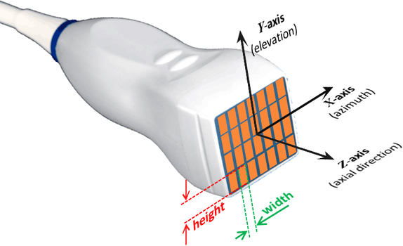
Conventional axes are used:
The X-axis is PARALLEL to the transducer. The Z-axis is PERPENDICULAR to the transducer and points downward (Z = 0 at the level of the transducer, Z increases as depth increases). The Y-axis is such that the coordinates are right-handed. These axes are represented in the above figure.
Element directivity
By default, the calculation is made faster by assuming that the directivity of the elements is dependent only on the central frequency (see figure below). This simplification very little affects the pressure field in most situations (except in the vicinity of the array). To turn off this option, use OPTIONS.FullFrequencyDirectivity = true.
See ADVANCED OPTIONS below.
Present version of PFIELD3
The present version of PFIELD3 only considers planar 2-D array whose z-coordinates of the elements are 0. All the elements are rectangular and have equal width and height.
PFIELD vs. PFIELD3
PFIELD and SIMUS use 2-D or 3-D linear acoustic equations depending on the input parameters. With PFIELD or SIMUS, a 3-D method is used to account for elevation focusing. The transmit delays in the Y direction cannot be adjusted as needed; only the elevation focal length can be modified. For more general 3-D cases, it is necessary to use PFIELD3 or SIMUS3.
Note on CHIRP signals
Linear chirps are characterized by PARAM.TXnow, PARAM.fc and PARAM.TXfreqsweep. The transmitted pulse has a duration of approximately T (= PARAM.TXnow/PARAM.fc), with the amplitude and phase defined over the time interval -T/2 to +T/2.
The total frequency sweep is DeltaF (= PARAM.TXfreqsweep): the frequencies increase linearly from (PARAM.fc - DeltaF/2) to (PARAM.fc + DeltaF/2) in the defined time interval.
Documentation: Chirp spectrum in Wikipedia.
Advanced options
- FREQUENCY SAMPLES
Only frequency components of the transmitted signal in the range [0, 2fc] with significant amplitude are considered. The default relative amplitude is -60 dB in PFIELD3. You can change this value by using the following:
[...] = PFIELD3(...,OPTIONS),
where OPTIONS.dBThresh is the threshold in dB (default = -60).
- FULL-FREQUENCY DIRECTIVITY
By default, the directivity of the elements depends on the center frequency only. This makes the algorithm faster. To make the directivities fully frequency-dependent, use:
[...] = PFIELD3(...,OPTIONS),
with OPTIONS.FullFrequencyDirectivity = true (default = false).
- ELEMENT SPLITTING
Each transducer element of the array is split into small rectangles. The width and height and of these small rectangles must be small enough to ensure that the far-field model is accurate. By default, the elements are split into M-by-|N| rectangles, with M and N being defined by:
M = ceil(element_width/smallest_wavelength); N = ceil(element_height/smallest_wavelength);
To modify the number MN of subelements by splitting, you may adjust OPTIONS.ElementSplitting, which must contain two elements. For example, OPTIONS.ElementSplitting = [1 3].
- WAIT BAR
If OPTIONS.WaitBar is true, a wait bar appears (only if the number of frequency samples >10). Default is true.
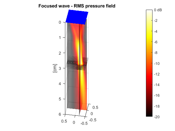
Example #1: 3-D focused pressure field with a matrix-array transducer
This example shows how to generate a three-dimensional focused pressure field with a matrix-array transducer.
Create a 3-MHz matrix array with 32x32 elements.
param = [];
param.fc = 3e6;
param.bandwidth = 70;
param.width = 250e-6;
param.height = 250e-6;
Specify the x- and y-coordinates of the elements.
pitch = 300e-6; % pitch (in m)
[xe,ye] = meshgrid(((1:32)-16.5)*pitch);
param.elements = [xe(:).'; ye(:).'];
Choose a focus point at xf = 0 mm, yf = -2 mm, zf = 30 mm.
xf = 0; yf = -2e-3; zf = 30e-3; % focus position (in m)
Obtain the corresponding transmit time delays with TXDELAY3.
txdel = txdelay3(xf,yf,zf,param); % in s
Simulate the pressure field by using PFIELD3.
First define a volume grid.
n = 32;
x = linspace(-5e-3,5e-3,n); % (in m)
y = linspace(-5e-3,5e-3,n); % (in m)
z = linspace(0,6e-2,4*n); % (in m)
[x,y,z] = meshgrid(x,y,z);
The function PFIELD3 yields the root-mean-square (RMS) pressure field.
RP = pfield3(x,y,z,txdel,param);
Display the acoustic pressure field and the element centers.
RPdB = 20*log10(RP/max(RP(:))); % convert to dB
slice(x*1e2,y*1e2,z*1e2,RPdB,xf*1e2,yf*1e2,zf*1e2)
shading flat
colormap(hot), caxis([-20 0])
set(gca,'zdir','reverse'), axis equal
alpha color % some transparency
c = colorbar; c.YTickLabel{end} = '0 dB';
zlabel('[cm]')
title('Focused wave - RMS pressure field')
view(-80,40)
hold on
plot3(xe*1e2,ye*1e2,xe*0,'b.')
hold off
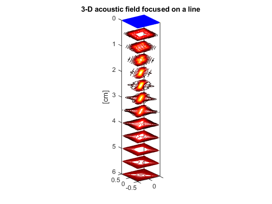
Example #2: 3-D pressure field focused on a line
This example shows how to generate a 3-D pressure field that focuses on a line with a matrix-array transducer.
Create a 3-MHz matrix array with 32x32 elements.
param = [];
param.fc = 3e6;
param.bandwidth = 70;
param.width = 250e-6;
param.height = 250e-6;
Specify the x- and y-coordinates of the elements.
pitch = 300e-6; % pitch (in m)
[xe,ye] = meshgrid(((1:32)-16.5)*pitch);
param.elements = [xe(:).'; ye(:).'];
Choose an oblique focus line by specifying two points.
xf = [-1e-2 1e-2]; % (in m)
yf = [-1e-2 1e-2]; % (in m)
zf = [2.5e-2 2.5e-2]; % (in m)
Obtain the corresponding transmit time delays (in s).
txdel = txdelay3(xf,yf,zf,param); % in s
Simulate the pressure field by using PFIELD3.
First define a volume grid.
n = 32;
x = linspace(-5e-3,5e-3,n); % (in m)
y = linspace(-5e-3,5e-3,n); % (in m)
z = linspace(0,6e-2,4*n); % (in m)
[x,y,z] = meshgrid(x,y,z);
The function PFIELD3 yields the root-mean-square (RMS) pressure field.
RP = pfield3(x,y,z,txdel,param);
Display the elements and the acoustic pressure field.
plot3(xe*1e2,ye*1e2,0*xe,'b.')
contourslice(x*1e2,y*1e2,z*1e2,RP,[],[],.5:.5:6,15)
set(gca,'zdir','reverse')
axis equal
colormap(hot)
zlabel('[cm]')
view(-35,20)
box on
title('3-D acoustic field focused on a line')
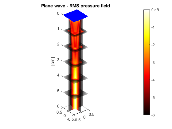
Example #3: Plane wave with a matrix array
This example shows how to simulate a plane wave with a matrix array.
Create a 3-MHz matrix array with 32x32 elements.
param = [];
param.fc = 3e6;
param.bandwidth = 70;
param.width = 250e-6;
param.height = 250e-6;
Specify the x- and y-coordinates of the elements.
pitch = 300e-6; % pitch (in m)
[xe,ye] = meshgrid(((1:32)-16.5)*pitch);
param.elements = [xe(:).'; ye(:).'];
Define a transmit apodization.
h = cos(linspace(-pi/4,pi/4,32));
h = h'*h;
param.TXapodization = h(:);
Choose the tilt angles about the X- and Y-axes.
tiltX = 0; % (in rad)
tiltY = 0; % (in rad)
Obtain the corresponding transmit time delays (in s).
txdel = txdelay3(param,tiltX,tiltY); % in s
Simulate the pressure field by using PFIELD3.
First define a volume grid.
n = 32;
x = linspace(-5e-3,5e-3,n); % (in m)
y = linspace(-5e-3,5e-3,n); % (in m)
z = linspace(0,6e-2,4*n); % (in m)
[x,y,z] = meshgrid(x,y,z);
The function PFIELD3 yields the root-mean-square (RMS) pressure field.
RP = pfield3(x,y,z,txdel,param);
Display the acoustic pressure field and the element centers.
RPdB = 20*log10(RP/max(RP(:))); % convert to dB
slice(x*1e2,y*1e2,z*1e2,RPdB,0,0,1:5)
shading flat
colormap(hot), caxis([-6 0])
set(gca,'zdir','reverse'), axis equal
% Fine-tune the figure:
alpha color % some transparency
c = colorbar; c.YTickLabel{end} = '0 dB';
zlabel('[cm]')
title('Plane wave - RMS pressure field')
hold on
plot3(xe*1e2,ye*1e2,xe*0,'b.')
hold off
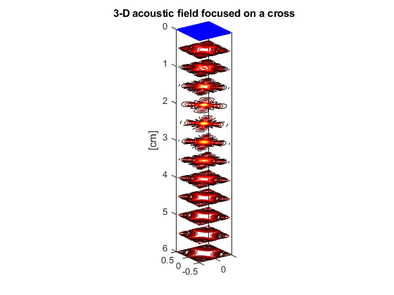
Example #4: Double-focus-line transmit with a matrix-array
This example shows how to generate a 3-D pressure field that focuses on a cross (two lines) with a matrix-array transducer.
Create a 3-MHz matrix array with 32x32 elements.
param = [];
param.fc = 3e6;
param.bandwidth = 70;
param.width = 250e-6;
param.height = 250e-6;
Specify the x- and y-coordinates of the elements.
pitch = 300e-6; % pitch (in m)
[xe,ye] = meshgrid(((1:32)-16.5)*pitch);
param.elements = [xe(:).'; ye(:).'];
Define two oblique focus line by specifying their points points.
xf1 = [-1e-2 1e-2]; % (in m)
yf1 = xf1; % (in m)
zf1 = [2.5e-2 2.5e-2]; % (in m)
xf2 = xf1; % (in m)
yf2 = -xf2; % (in m)
zf2 = zf1; % (in m)
Obtain the corresponding transmit time delays (in s).
txdel1 = txdelay3(xf1,yf1,zf1,param); % in s
txdel2 = txdelay3(xf2,yf2,zf2,param); % in s
Simulate the pressure field by using PFIELD3.
First define a volume grid.
n = 32;
x = linspace(-5e-3,5e-3,n); % (in m)
y = linspace(-5e-3,5e-3,n); % (in m)
z = linspace(0,6e-2,4*n); % (in m)
[x,y,z] = meshgrid(x,y,z);
The function PFIELD3 yields the root-mean-square (RMS) pressure field.
RP = pfield3(x,y,z,[txdel1;txdel2],param);
Display the elements and the acoustic pressure field.
plot3(xe*1e2,ye*1e2,0*xe,'b.')
contourslice(x*1e2,y*1e2,z*1e2,RP,[],[],.5:.5:6,15)
set(gca,'zdir','reverse')
% Fine-tune the figure:
axis equal
colormap(hot)
zlabel('[cm]')
view(-35,20)
box on
title('3-D acoustic field focused on a cross')
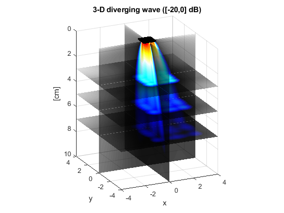
Example #5: 3-D diverging wave with a matrix array
This example shows how to generate a diverging pressure field with a matrix transducer.
Create a 3-MHz matrix array with 32x32 elements.
param = [];
param.fc = 3e6;
param.bandwidth = 70;
param.width = 250e-6;
param.height = 250e-6;
Specify the x- and y-coordinates of the elements.
pitch = 300e-6; % pitch (in m)
[xe,ye] = meshgrid(((1:32)-16.5)*pitch);
param.elements = [xe(:).'; ye(:).'];
Define a transmit apodization.
h = cos(linspace(-pi/4,pi/4,32));
h = h'*h;
param.TXapodization = h(:);
Generate the transmit time delays for a diverging wave.
tiltX = 10/180*pi; % tilt angle about the X-axis (in rad)
tiltY = 10/180*pi; % tilt angle about the Y-axis (in rad)
omega = 30/180*pi; % solid angle (in sr)
txdel = txdelay3(param,tiltX,tiltY,omega); % in s
Simulate the pressure field by using PFIELD3.
First define the x-, y-, z-coordinates of the ROI:
x = linspace(-4e-2,4e-2,200);
y = x;
z = linspace(0,10e-2,200);
Obtain the RMS pressure field on the azimuthal plane:
[xaz,zaz] = meshgrid(x,z);
yaz = zeros(size(xaz));
Paz = pfield3(xaz,yaz,zaz,txdel,param);
Obtain the RMS pressure field on the elevation plane:
[yel,zel] = meshgrid(y,z);
xel = zeros(size(yel));
Pel = pfield3(xel,yel,zel,txdel,param);
Obtain the RMS pressure field on some parallel planes:
[xfo,yfo] = meshgrid(x,y);
zfo1 = ones(size(xfo))*3e-2;
zfo2 = ones(size(xfo))*5e-2;
zfo3 = ones(size(xfo))*7e-2;
Pfo1 = pfield3(xfo,yfo,zfo1,txdel,param);
Pfo2 = pfield3(xfo,yfo,zfo2,txdel,param);
Pfo3 = pfield3(xfo,yfo,zfo3,txdel,param);
Display the acoustic pressure field.
Pmax = max(max(Paz(:)),max(Pel(:)));
surf(xaz*1e2,yaz*1e2,zaz*1e2,20*log10(Paz/Pmax)), shading flat
hold on
surf(xel*1e2,yel*1e2,zel*1e2,20*log10(Pel/Pmax)), shading flat
surf(xfo*1e2,yfo*1e2,zfo1*1e2,20*log10(Pfo1/Pmax)), shading flat
surf(xfo*1e2,yfo*1e2,zfo2*1e2,20*log10(Pfo2/Pmax)), shading flat
surf(xfo*1e2,yfo*1e2,zfo3*1e2,20*log10(Pfo3/Pmax)), shading flat
% Display the elements
plot3(xe*1e2,ye*1e2,xe*0,'k.')
hold off
% Fine-tune the figure:
axis equal
zlabel('[cm]')
set(gca,'ZDir','reverse')
title('3-D diverging wave ([-20,0] dB)')
caxis([-20 0])
alpha color
colormap(flipud([hot;1-hot]))
xlabel('x')
ylabel('y')
view(-25,20)
See also
cite, getparam, pfield, simus3, txdelay3, viewxdcr
References
- The paper that describes the first 2-D version of PFIELD is: Shariari S, Garcia D. Meshfree simulations of ultrasound vector flow imaging using smoothed particle hydrodynamics. Phys Med Biol, 2018;63:205011. (PDF)
- The papers that describe the theory inside PFIELD and SIMUS are: Garcia D. SIMUS: an open-source simulator for medical ultrasound imaging. Part I: theory & examples. Comput Methods Programs Biomed, 2022. (PDF), and: Cigier A, Varray F, Garcia D. SIMUS: an open-source simulator for medical ultrasound imaging. Part II: comparison with four simulators. Comput Methods Programs Biomed, 2022. (PDF).
- There is yet no publication for PFIELD3 (it is planned for 2023-24).
About the author
Damien Garcia, Eng., Ph.D.
INSERM researcher
Creatis, University of Lyon, France
websites: BioméCardio, MUST
Date modified