`TXDELAY3` Transmit delays for a matrix array

TXDELAY returns the transmit time delays for focused, plane or diverging beam patterns with a matrix array.

Syntax
The structure PARAM
Notes
Example #1: 3-D focused pressure field with a matrix-array transducer
Example #2: 3-D diverging wave with a matrix array
See also
About the author
Date modified

Syntax

DELAYS = TXDELAY3(X0,Y0,Z0,PARAM) returns the transmit time delays for a pressure field focused at the point (x0,y0,z0). If z0 is negative, then the point (x0,y0,z0) is a virtual source. The properties of the medium and array must be given in the structure PARAM (see below).

DELAYS = TXDELAY3([X01 X02],[Y01 Y02],[Z01 Z02],PARAM) returns the transmit time delays for a pressure field focused at the line specified by the two points (x01,y01,z01) and (x02,y02,z02).

DELAYS = TXDELAY3(PARAM,TILTx,TILTy) returns the transmit time delays for a tilted plane wave. TILTx is the tilt angle about the X-axis. TILTy is the tilt angle about the Y-axis. If TILTx = TILTy = 0, then the delays are 0.

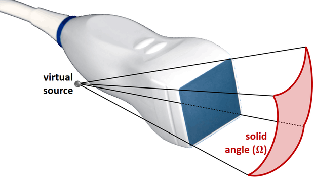
DELAYS = TXDELAY3(PARAM,TILTx,TILTy,OMEGA) yields the transmit time delays for a diverging wave. The sector is characterized by the angular tilts and the solid angle OMEGA subtented by the rectangular aperture of the transducer. TILTx is the tilt angle about the X-axis. TILTy is the tilt angle about the Y-axis. OMEGA sets the amount of the field of view (in [0 2pi]). This syntax is for matrix arrays only, i.e. the element positions must form a plaid grid.

[DELAYS,PARAM] = TXDELAY3(...) updates the PARAM structure parameters including the default values. PARAM will also include PARAM.TXdelay, which is equal to DELAYS (in s).

[...] = TXDELAY3 (no input parameter) simulates a focused pressure field generated by a 3-MHz 32x32 matrix array (1st example below).

Units: X0, Y0 and Z0 must be in m; TILTx and TILTy must be in rad. OMEGA is in sr (steradian). DELAYS are in s.

The structure `PARAM`

PARAM is a structure that must contain the following fields:

PARAM.elements: x- and y-coordinates of the element centers (in m, required). It MUST be a two-row matrix, with the 1st and 2nd rows containing the x and y coordinates, respectively.
PARAM.width: element width, in the x-direction (in m, required)
PARAM.height: element height, in the y-direction (in m, required)
PARAM.c: longitudinal velocity (in m/s, default = 1540 m/s)

Notes

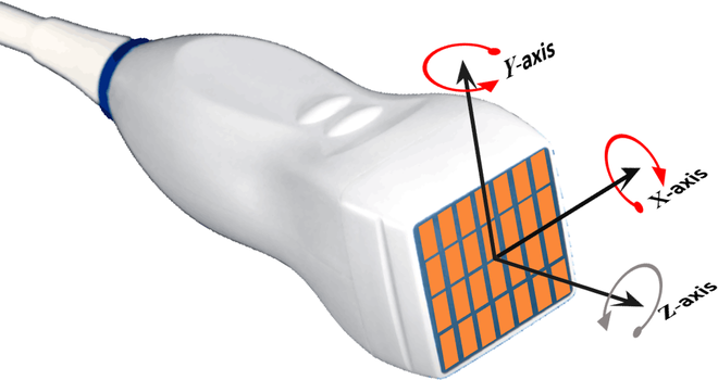
NOTE #1: X-, Y-, and Z-axes

For a linear array, the X-axis is PARALLEL to the transducer and points from the first (leftmost) element to the last (rightmost) element (X = 0 at the CENTER of the transducer).

The Z-axis is PERPENDICULAR to the transducer and points downward (Z = 0 at the level of the transducer, Z increases as depth increases). See the figure below.

The Y-axis is is such that the coordinates are right-handed.

NOTE #2: TILT angles

TILTx and TILTy (in radians) describe the tilt angles in the trigonometric direction.

NOTE #3: solid angle OMEGA

For a diverging wave with a matrix array, OMEGA describes the solid angle subtented by the rectangular aperture of the transducer.

Example #1: 3-D focused pressure field with a matrix-array transducer

This example shows how to generate a three-dimensional focused pressure field with a matrix-array transducer.

Create a 3-MHz matrix array with 32x32 elements.

param = [];
param.fc = 3e6;
param.bandwidth = 70;
param.width = 250e-6;
param.height = 250e-6;

Specify the x- and y-coordinates of the elements.

pitch = 300e-6; % pitch (in m)
[xe,ye] = meshgrid(((1:32)-16.5)*pitch);
param.elements = [xe(:).'; ye(:).'];

Choose a focus point at xf = 0 mm, yf = -2 mm, zf = 30 mm.

xf = 0; yf = -2e-3; zf = 30e-3; % focus position (in m)

Obtain the corresponding transmit time delays with TXDELAY3.

txdel = txdelay3(xf,yf,zf,param); % in s

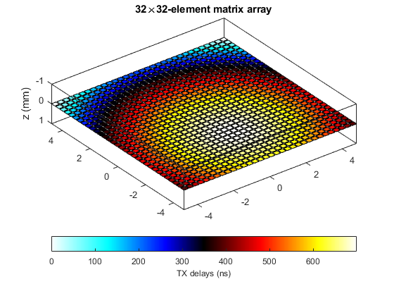
Check the elements and the delays with VIEWXDCR

p = viewxdcr(param);
p.FaceVertexCData = txdel(:)*1e9;
c = colorbar('SouthOutside');
c.Label.String = 'TX delays (ns)';
colormap([1-hot;hot])
title('32\times32-element matrix array')

Simulate the pressure field by using PFIELD3.

First define a volume grid.

n = 32;
x = linspace(-5e-3,5e-3,n); % (in m)
y = linspace(-5e-3,5e-3,n); % (in m)
z = linspace(0,6e-2,4*n); % (in m)
[x,y,z] = meshgrid(x,y,z);

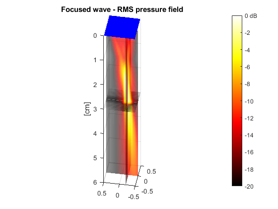
The function PFIELD3 yields the root-mean-square (RMS) pressure field.

RP = pfield3(x,y,z,txdel,param);

Display the acoustic pressure field and the element centers.

RPdB = 20*log10(RP/max(RP(:))); % convert to dB
slice(x*1e2,y*1e2,z*1e2,RPdB,xf*1e2,yf*1e2,zf*1e2)
shading flat
colormap(hot), caxis([-20 0])
set(gca,'zdir','reverse'), axis equal
alpha color % some transparency
c = colorbar;
c.YTickLabel{end} = '0 dB';
zlabel('[cm]')
title('Focused wave - RMS pressure field')
view(-80,40)
hold on
plot3(xe*1e2,ye*1e2,xe*0,'b.')
hold off

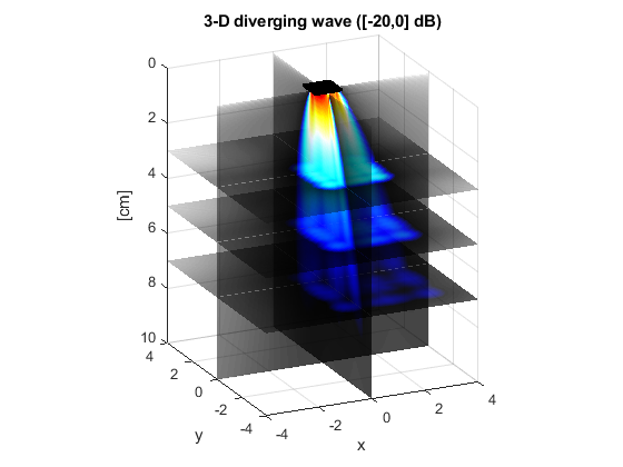
Example #2: 3-D diverging wave with a matrix array

This example shows how to generate a diverging pressure field with a matrix transducer.

Create a 3-MHz matrix array with 32x32 elements.

param = [];
param.fc = 3e6;
param.bandwidth = 70;
param.width = 250e-6;
param.height = 250e-6;

Specify the x- and y-coordinates of the elements.

pitch = 300e-6; % pitch (in m)
[xe,ye] = meshgrid(((1:32)-16.5)*pitch);
param.elements = [xe(:).'; ye(:).'];

Define a transmit apodization.

h = cos(linspace(-pi/4,pi/4,32));
h = h'*h;
param.TXapodization = h(:);

Generate the transmit time delays for a diverging wave with TXDELAY3.

tiltX = 10/180*pi; % tilt angle about the X-axis (in rad)
tiltY = 10/180*pi; % tilt angle about the Y-axis (in rad)
omega = 30/180*pi; % solid angle (in sr)
txdel = txdelay3(param,tiltX,tiltY,omega); % in s

Check the elements and the delays with VIEWXDCR

delete(gcf); % delete the current figure
p = viewxdcr(param);
p.FaceVertexCData = txdel(:)*1e6;
c = colorbar('SouthOutside');
c.Label.String = 'TX delays (ms)';
colormap([1-hot;hot])
title('32\times32-element matrix array')

Simulate the pressure field by using PFIELD3.

First define the x-, y-, z-coordinates of the ROI:

x = linspace(-4e-2,4e-2,200);
y = x;
z = linspace(0,10e-2,200);

Obtain the RMS pressure field on the azimuthal plane:

[xaz,zaz] = meshgrid(x,z);
yaz = zeros(size(xaz));
Paz = pfield3(xaz,yaz,zaz,txdel,param);

Obtain the RMS pressure field on the elevation plane:

[yel,zel] = meshgrid(y,z);
xel = zeros(size(yel));
Pel = pfield3(xel,yel,zel,txdel,param);

Obtain the RMS pressure field on some parallel planes:

[xfo,yfo] = meshgrid(x,y);
zfo1 = ones(size(xfo))*3e-2;
zfo2 = ones(size(xfo))*5e-2;
zfo3 = ones(size(xfo))*7e-2;
Pfo1 = pfield3(xfo,yfo,zfo1,txdel,param);
Pfo2 = pfield3(xfo,yfo,zfo2,txdel,param);
Pfo3 = pfield3(xfo,yfo,zfo3,txdel,param);

Display the acoustic pressure field.

Pmax = max(max(Paz(:)),max(Pel(:)));
surf(xaz*1e2,yaz*1e2,zaz*1e2,20*log10(Paz/Pmax)), shading flat
hold on
surf(xel*1e2,yel*1e2,zel*1e2,20*log10(Pel/Pmax)), shading flat
surf(xfo*1e2,yfo*1e2,zfo1*1e2,20*log10(Pfo1/Pmax)), shading flat
surf(xfo*1e2,yfo*1e2,zfo2*1e2,20*log10(Pfo2/Pmax)), shading flat
surf(xfo*1e2,yfo*1e2,zfo3*1e2,20*log10(Pfo3/Pmax)), shading flat
% Display the elements
plot3(xe*1e2,ye*1e2,xe*0,'k.')
hold off
% Fine-tune the figure:
axis equal
zlabel('[cm]')
set(gca,'ZDir','reverse')
title('3-D diverging wave ([-20,0] dB)')
caxis([-20 0])
alpha color
colormap(flipud([hot;1-hot]))
xlabel('x')
ylabel('y')
view(-25,20)

About the author

Damien Garcia, Eng., Ph.D.
INSERM researcher
Creatis, University of Lyon, France

websites: BioméCardio, MUST

TXDELAY3 Transmit delays for a matrix array

Contents