DASMTX3 Delay-And-Sum matrix for 3-D imaging
DASMTX3 returns a Delay-And-Sum matrix for linear 3-D beamforming.
Contents
Syntax
M = DASMTX3(SIG,X,Y,Z,DELAYS,PARAM) returns the numel(X) -by- numel(SIG) delay-and-sum DAS matrix. The matrix M can be used to beamform SIG (RF or I/Q signals) at the points specified by X, Y, and Z.
Because the signals in SIG are not required (only its size is needed) to create M, the following syntax is recommended:
M = DASMTX3(size(SIG),X,Y,Z,DELAYS,PARAM)
!IMPORTANT! -- With this syntax, use M = DASMTX3(1i*size(SIG),...) to return a complex DAS matrix for I/Q data.
DELAYS are the transmit time delays (in s). The number of elements in DELAYS must be the number of elements in the array (which is equal to size(SIG,2)). If a sub-aperture was used during transmission, use DELAYS(i) = NaN if element # i of the linear array was off.
PARAM is a structure that contains the parameter values required for DAS beamforming (see below for details).
DASMTX3 versus DAS3
DASMTX3 is called by DAS3. DASMTX3 thus returns the same beamformed results as DAS3.
- Beamforming using DAS3:
bfSIG = das3(SIG,x,y,z,delays,param)
- Beamforming using DASMTX3:
M = dasmtx3(size(SIG),x,y,z,delays,param);
bfSIG = M*SIG(:);
bfSIG = reshape(bfSIG,size(x));
M is a large sparse matrix. Computing M can be much more cost-effective than using DAS if you need to beamform several SIG matrices, because M needs to be determined only once. In 3-D ultrasound imaging with a significant number of elements, however, DASMTX3 can generate tall sparse DAS matrices when beamforming large volume data! To avoid memory issues, consider chunking your datasets to create several smaller sparse matrices.
Let us consider that a series SIG{1}, SIG{2} ... SIG{N} of ultrasound matrices have been generated by sending similar wavefronts with the same ultrasound array. These signals SIG{i} are stacked in a 3D array sig3D so that sig3D(:,:,i) = SIG{i}. To beamform these data with a delay-and-sum approach, the following can be used.
To obtain the DAS matrix, use dasmtx3:
M = dastmtx3([size(sig3D,1) size(sig3D,2)],x,y,z,delays,param) or
M = dastmtx3(1i*[size(sig3D,1) size(sig3D,2)],...) for I/Q data.
The beamformed signals are then calculated by a matrix multiplication:
bfSIG3D = M*reshape(sig3D,[],size(sig3D,3))
It is necessary to reshape the beamformed matrix array:
bfSIG3D = reshape(bfSIG3D,size(x,1),size(x,2),[])
You can also consider saving the DAS matrix M in a MAT file and loading it when needed. The previous syntax is generally much faster than:
for k = 1:N, bfSIG{k} = das3(SIG{k},x,y,z,delays,param); end
Other syntaxes
DASMTX3(SIG,X,Y,Z,PARAM) uses DELAYS = param.TXdelay.
DASMTX3(...,METHOD) specifies the interpolation method. The available methods are decribed in NOTE #3 below.
[M,PARAM] = DASMTX3(...) also returns the structure PARAM with the default values.
The structure PARAM
PARAM is a structure that contains the following fields:
- PARAM.fs: sampling frequency (in Hz, required)
- PARAM.elements: x- and y-coordinates of the element centers (in m, required). It MUST be a two-row matrix, with the 1st and 2nd rows containing the x and y coordinates, respectively.
- PARAM.fc: central frequency (in Hz, required for I/Q signals)
- PARAM.TXdelay: transmission law delays (in s, required if the vector DELAYS is not given)
- PARAM.c: longitudinal velocity (in m/s, default = 1540 m/s)
- PARAM.t0: start time for reception (in s, default = 0 s)
- PARAM.fnumber: reception f-number (default = [0 0], i.e. full aperture). PARAM.fnumber(1) = reception f-number in the azimuthal x-direction. PARAM.fnumber(2) = reception f-number in the elevation y-direction.
Notes
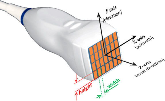
- NOTE #1: X-, Y-, and Z-axes
Conventional axes are used:
The X-axis is PARALLEL to the transducer. The Z-axis is PERPENDICULAR to the transducer and points downward (Z = 0 at the level of the transducer, Z increases as depth increases). The Y-axis is such that the coordinates are right-handed. These axes are represented in the following figure.
- NOTE #2:
DASMTX3 uses a standard delay-and-sum. It is a linear operator. Phase rotations are included if I/Q (complex) signals are beamformed.
- NOTE #3: interpolation methods
By default DASMTX3 uses a linear interpolation to generate the DAS matrix. To specify the interpolation method, use DASMTX3(...,METHOD), with METHOD being:
- 'nearest' : nearest neighbor interpolation
- 'linear' : (default) linear interpolation
- 'quadratic' : quadratic interpolation
- 'lanczos3' : 3-lobe Lanczos (windowed sinc) interpolation
- '5points' : 5-point least-squares parabolic interpolation
- 'lanczos5' : 5-lobe Lanczos (windowed sinc) interpolation
The linear interpolation (it is a 2-point method) returns a matrix twice denser than the nearest-neighbor interpolation. It is 3, 4, 5, 6 times denser for 'quadratic', 'lanczos3', '5points', 'lanczos5', respectively (they are 3-to-6-point methods).
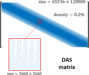
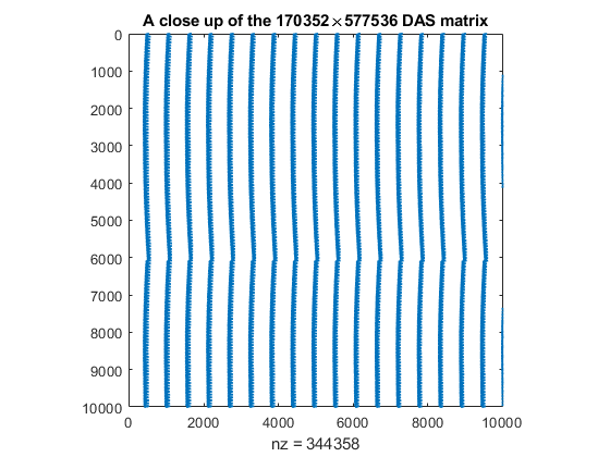
The DAS matrix
The DAS matrix is very sparse. It is complex when beamforming I/Q signals, which should be the preferred approach.
Here is an example of a DAS matrix:
Example: Two-way PSF for a focused wave by a 32x32 matrix array
This example shows how to simulate RF signals then beamform I/Q signals
Create a 3-MHz matrix array with 32x32 elements.
param = [];
param.fc = 3e6;
param.bandwidth = 70;
param.width = 250e-6;
param.height = 250e-6;
Specify the x- and y-coordinates of the elements.
pitch = 300e-6; % pitch (in m)
[xe,ye] = meshgrid(((1:32)-16.5)*pitch);
param.elements = [xe(:).'; ye(:).'];
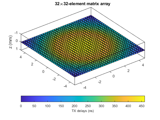
Use TXDELAY3 to calculate the transmit delays for a focused wave.
x0 = 0; y0 = 0; z0 = 3e-2;
txdel = txdelay3(x0,y0,z0,param);
Plot the transducer with VIEWXDCR.
p = viewxdcr(param);
p.FaceVertexCData = txdel(:)*1e9;
title('32\times32-element matrix array')
c = colorbar('SouthOutside');
c.Label.String = 'TX delays (ns)';
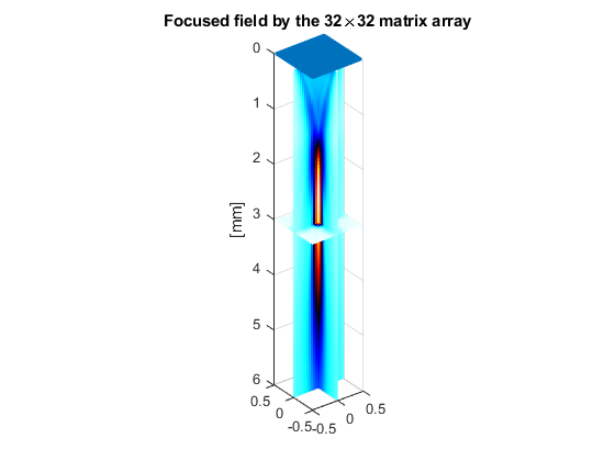
Calculate the pressure field with PFIELD3.
n = 24;
[xi,yi,zi] = meshgrid(linspace(-5e-3,5e-3,n),linspace(-5e-3,5e-3,n),...
    linspace(0,6e-2,4*n));
RP = pfield3(xi,yi,zi,txdel,param);
Have a look at the RMS pressure field.
figure
slice(xi*1e2,yi*1e2,zi*1e2,RP,0,0,3)
set(gca,'zdir','reverse')
zlabel('[mm]')
shading flat
axis equal
colormap([1-hot;hot])
hold on
plot3(xe(:)*1e2,ye(:)*1e2,0*xe(:),'.')
title('Focused field by the 32{\times}32 matrix array')
Simulate RF signals by using SIMUS3.
[RF,param] = simus3(x0,y0,z0,1,txdel,param);
Demodulate the RF signals with RF2IQ.
IQ = rf2iq(RF,param);
Create a 3-D grid for beamforming.
lambda = 1540/param.fc;
[xi,yi,zi] = meshgrid(-2e-2:lambda:2e-2,-2e-2:lambda:2e-2,...
    2.5e-2:lambda/2:3.2e-2);
Create the DAS matrix with DASMTX3.
M = dasmtx3(1i*size(IQ),xi,yi,zi,txdel,param);
figure
spy(M(1:10000,1:10000))
title(['A close up of the ' int2str(size(M,1)) '\times',...
    int2str(size(M,2)) ' DAS matrix'])
Beamform the I/Q signals.
IQb = M*IQ(:);
IQb = reshape(IQb,size(xi));
Obtain the log-envelope.
env = abs(IQb);
I = 20*log10(env/max(env(:)));
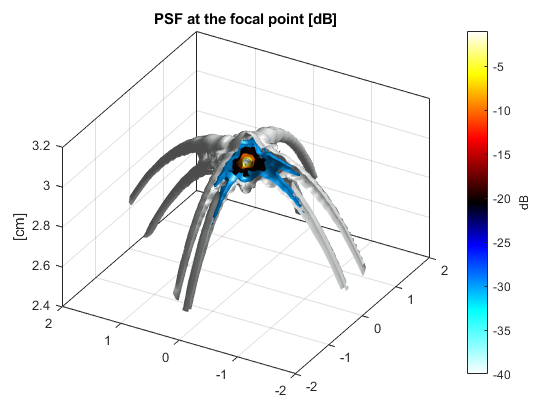
Display the two-way PSF.
figure
I(1:round(size(I,1)/2),1:round(size(I,2)/2),:) = NaN;
for k = [-40:10:-10 -5 -1]
    isosurface(xi*1e2,yi*1e2,zi*1e2,I,k)
end
view(-60,40)
colormap([1-hot;hot])
c = colorbar;
c.Label.String = 'dB';
box on, grid on
zlabel('[cm]')
title('PSF at the focal point [dB]')
See also
cite, das3, dasmtx, simus3, txdelay3
References
- Perrot V, Polichetti M, Varray F, Garcia D. So you think you can DAS? A viewpoint on delay-and-sum beamforming. Ultrasonics, 2021; 111:106309. (PDF)
- If you use PARAM.RXangle for vector Doppler: Madiena C, Faurie J, Porée J, Garcia D. Color and vector flow imaging in parallel ultrasound with sub-Nyquist sampling. IEEE TUFFC, 2018;65:795-802. (PDF)
About the author
Damien Garcia, Eng., Ph.D.
INSERM researcher
Creatis, University of Lyon, France
websites: BioméCardio, MUST
Date modified